Pseudo-bulk Vignette
Vittoria Martinolli D’Arcy, Alexander Yermanos
30/05/2022
Source:vignettes/pseudo_bulk.Rmd
pseudo_bulk.Rmd1. Setup
First of all the vgm data is obtained downloading the raw data and converting into the VDJ_GEX_matrix structure.
2. Function usage and examples
The pseudo_bulk_DE function takes a VGM object as an input and performs pseudo-bulk on the data, according to criteria specified by the User. Differential Gene Expression (DGE) analysis is then performed on the pseudo-bulked data. The output is a data.frame or list of data.frames containing the results of the DGE analysis for every level of pseudo-bulking. In particular three different options are available for pseudo-bulking the samples:
2.1 Two different pseduo-bulking categories
Choosing one VGM column (column.group) from where to pick two samples or two groups of samples to test for DGE. In parallel choosing another column (column.comparison) of the VGM object from where to pick the “levels of comparison”, meaning that the two samples picked in the first column will be tested against each other across the categories picked in the second column, separating the analysis and results according to each cathegory.
pseudo_DE<-GEX_pseudobulk(vgm.input=VGM_NP396_GP33_GP66_labelled, column.group="sample_id", group1 = c("s1"), group2 = c( "s4"), column.comparison = "seurat_clusters", comparison=c(2,3,5,9), pool=FALSE)The output is a list of data.frames each including the results of the DGE analysis of the respecitive comparison level.
pseudo_DE[[2]]## logFC logCPM LR p_val p_adj gene
## XIST -10.558188 7.109666 30.28749 3.725201e-08 0.0004881503 XIST
## TTR 6.851042 7.985671 26.41093 2.759747e-07 0.0012456126 TTR
## UTY 9.789416 6.354439 26.34764 2.851677e-07 0.0012456126 UTY
## CD200R1 8.945437 5.546191 21.41346 3.701633e-06 0.0097012385 CD200R1
## DDX3Y 8.945437 5.546191 21.41346 3.701633e-06 0.0097012385 DDX3Y
## EIF2S3Y 8.844367 5.450930 20.83781 4.998646e-06 0.0109170433 EIF2S3Y
## COCH 8.490147 5.120463 18.85308 1.411827e-05 0.0264293922 COCH
## DSCAM 8.421630 5.057220 18.47565 1.720893e-05 0.0281882270 DSCAM
## GLRX5 -8.406211 5.060621 17.81171 2.438775e-05 0.0355085710 GLRX5
## FGL2 4.815742 7.186576 16.33124 5.317987e-05 0.0640682581 FGL2
## CDH1 8.019631 4.691409 16.30993 5.378135e-05 0.0640682581 CDH1
## SEMA6D 5.644681 5.399101 15.44681 8.486014e-05 0.0926672692 SEMA6D
## comparison_id
## XIST comparison_2
## TTR comparison_2
## UTY comparison_2
## CD200R1 comparison_2
## DDX3Y comparison_2
## EIF2S3Y comparison_2
## COCH comparison_2
## DSCAM comparison_2
## GLRX5 comparison_2
## FGL2 comparison_2
## CDH1 comparison_2
## SEMA6D comparison_2
pseudo_DE[[4]]## logFC logCPM LR p_val p_adj gene
## CCR7 8.657396 7.989358 31.12190 2.423220e-08 0.0002511667 CCR7
## SCGB1C1 8.229789 7.573113 26.73656 2.331679e-07 0.0012083926 SCGB1C1
## ACTA2 7.922810 7.280981 23.74721 1.098544e-06 0.0037954689 ACTA2
## LYZ2 4.323782 8.711587 21.72485 3.146889e-06 0.0081543752 LYZ2
## SLCO1A4 7.119907 6.558915 16.72673 4.316841e-05 0.0745734286 SLCO1A4
## TTR 7.119907 6.558915 16.72673 4.316841e-05 0.0745734286 TTR
## SERPINB6B -7.667660 7.352629 15.81782 6.974257e-05 0.0829426574 SERPINB6B
## LY6C1 6.995319 6.454071 15.75703 7.201967e-05 0.0829426574 LY6C1
## XIST -7.710520 7.388403 16.11945 5.947026e-05 0.0829426574 XIST
## comparison_id
## CCR7 comparison_9
## SCGB1C1 comparison_9
## ACTA2 comparison_9
## LYZ2 comparison_9
## SLCO1A4 comparison_9
## TTR comparison_9
## SERPINB6B comparison_9
## LY6C1 comparison_9
## XIST comparison_9In the output object there is also a summary indicating the correspondences between samples, groups and comparison levels.
pseudo_DE[["summary"]]## DataFrame with 8 rows and 4 columns
## sample_id comparison groups levels
## <character> <factor> <factor> <character>
## s1_AAACCTGCAAGCTGGA-1 s1 comparison_3 group1 group1_comparison_3
## s1_AAACCTGGTGCTCTTC-1 s1 comparison_2 group1 group1_comparison_2
## s1_AAACGGGGTATTCTCT-1 s1 comparison_5 group1 group1_comparison_5
## s1_AACTCAGCAAGCCGTC-1 s1 comparison_9 group1 group1_comparison_9
## s4_AAACCTGGTGCTGTAT-1 s4 comparison_5 group2 group2_comparison_5
## s4_AAACCTGGTTGACGTT-1 s4 comparison_3 group2 group2_comparison_3
## s4_AAACCTGTCACGGTTA-1 s4 comparison_2 group2 group2_comparison_2
## s4_AAAGATGGTGCCTGTG-1 s4 comparison_9 group2 group2_comparison_9pseudo_DE[[“number_de”]] reports the percentages and numbers of defferentially expressed genes per comparison level.
pseudo_DE[["number_de"]]## number_de percentage_de
## [1,] 86 0.27145608
## [2,] 12 0.03787759
## [3,] 77 0.24304788
## [4,] 9 0.028408192.2 One pseudo-bulking category. Pooling samples together into two groups.
Choosing one VGM column only (column.group), from which to pick two groups of samples to test for DGE and pooling together all the samples belonging to the first group as group1 and all the samples belonging to the second group as group2. Group1 and group2 will be tested against each other. This option is allowed by setting pool=TRUE.
pseudo_DE_pooled<-GEX_pseudobulk(vgm.input=VGM_NP396_GP33_GP66_labelled, column.group="sample_id", group1 = c("s1", "s2"), group2 = c("s4", "s3"), column.comparison = NULL, comparison=NULL, pool=TRUE)

head(pseudo_DE_pooled)
## logFC logCPM LR p_val p_adj
## XIST -11.038506 7.131469 324.7100 1.364543e-72 2.749965e-68
## UTY 13.446177 5.272431 255.2942 1.820980e-57 1.834910e-53
## EIF2S3Y 9.865577 5.641570 249.4288 3.459111e-56 2.323716e-52
## DDX3Y 9.994586 5.171616 236.4760 2.307404e-53 1.162528e-49
## KDM5D 11.382699 3.235047 165.9324 5.723002e-38 2.306713e-34
## 3830403N18RIK -8.916710 2.922212 160.7510 7.754915e-37 2.604747e-33
## gene
## XIST XIST
## UTY UTY
## EIF2S3Y EIF2S3Y
## DDX3Y DDX3Y
## KDM5D KDM5D
## 3830403N18RIK 3830403N18RIK2.3 One pseudo-bulking category. Separating samples within the same group.
Choosing one VGM column only (column.group), from which to pick two groups of samples to test for DGE and NOT pooling together samples belonging to the same group. A pairwise DGE analysis between the samples of group1 and sample of group2 is performed, therfore the order accoring to which the samples are inserted in the input matters. This option is allowed by setting pool=FALSE
pseudo_DE_clusters<-GEX_pseudobulk(vgm.input=VGM_NP396_GP33_GP66_labelled, column.group="seurat_clusters", group1 = c(2,4,6), group2 = c(1,3,9), pool=FALSE)

head(pseudo_DE_clusters[[1]])
## logFC logCPM LR p_val p_adj gene
## ASCL2 -8.842313 2.758881 64.00282 1.242410e-15 1.297413e-11 ASCL2
## SOSTDC1 -6.733771 7.309354 63.91531 1.298842e-15 1.297413e-11 SOSTDC1
## GM47957 -7.864154 2.706008 59.26261 1.379734e-14 9.188111e-11 GM47957
## CD83 -6.224031 4.578687 54.63028 1.454767e-13 7.265833e-10 CD83
## GM4208 7.081434 2.326647 53.25790 2.925094e-13 1.168751e-09 GM4208
## GAL -10.373562 1.071609 48.54325 3.230840e-12 1.075762e-08 GAL
## comparison_id
## ASCL2 comparison_1
## SOSTDC1 comparison_1
## GM47957 comparison_1
## CD83 comparison_1
## GM4208 comparison_1
## GAL comparison_1
pseudo_DE_clusters[["summary"]]## DataFrame with 6 rows and 3 columns
## seurat_clusters comparison groups
## <factor> <factor> <factor>
## s1_AAACCTGCAAGCTGGA-1 3 comparison_2 group2
## s1_AAACCTGCACCAGTTA-1 1 comparison_1 group2
## s1_AAACCTGCATCGGTTA-1 6 comparison_3 group1
## s1_AAACCTGGTGCTCTTC-1 2 comparison_1 group1
## s1_AAACGGGAGAATGTTG-1 4 comparison_2 group1
## s1_AACTCAGCAAGCCGTC-1 9 comparison_3 group2#3. Plots
Plotting option is not included in the function, but plots can be generated with the following few lines of code, to be adapted according to the data.
##3.1 Violin Plot
##Violin Plot

# pull top-n genes for each cluster
top_gs <- list()
top_gs$comparison_3 <- pseudo_DE[[1]]$gene[seq_len(9)]
top_gs$comparison_2 <- pseudo_DE[[2]]$gene[seq_len(9)]
top_gs$comparison_5 <- pseudo_DE[[3]]$gene[seq_len(9)]
top_gs$comparison_9 <- pseudo_DE[[4]]$gene[seq_len(9)]

# get top gene-hits common among clusters, or genes the user is interested in plotting
top_gs$common <- c("XIST" ,"TTR" ,"UTY", "DDX3Y", "EIF2S3Y",  "COCH", "CCR7" , "DSCAM")

# split cells by cluster
cs_by_k <- split(colnames(input),input@colData@listData[["comparison"]])

#plot violin plot including all the comparison levels in the same plot

pseudo_bulk_all_fig<-scater::plotExpression(input, features = top_gs$common,
        x = "levels", colour_by = "groups", ncol = 2) +
        guides(fill = guide_legend(override.aes = list(size = 5, alpha = 1))) +
        theme_classic() + theme(axis.text.x = element_text(angle = 45, hjust = 1))
pseudo_bulk_all_fig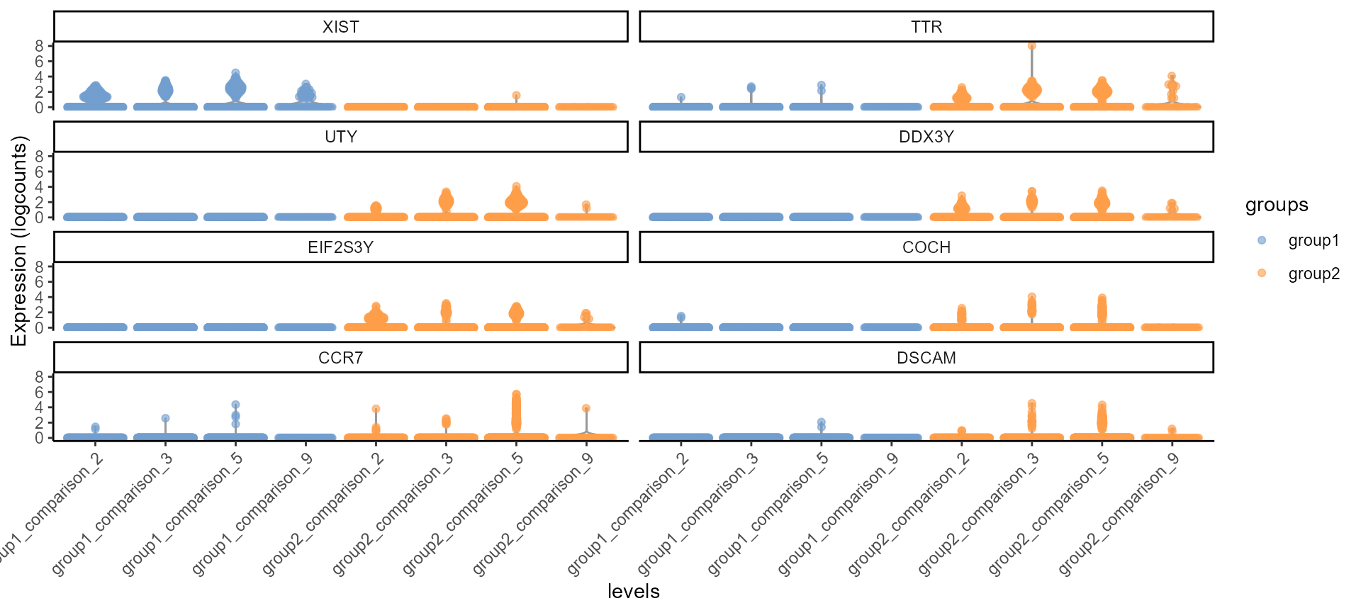
Violin Plot, including all the comparison levels in the same plot.
#otherwise plot violin plot by comparison level k

gs <- top_gs[["comparison_3"]]  # get top gene-hits for comparison k
cs <- cs_by_k[["comparison_3"]] # subset cells assigned to comparison k
comparison_3.fig<-scater::plotExpression(input[,cs], features = gs,
        x = "levels", colour_by = "groups", ncol = 3) +
        guides(fill = guide_legend(override.aes = list(size = 5, alpha = 1))) +
        theme_classic() + theme(axis.text.x = element_text(angle = 45, hjust = 1))

plot(comparison_3.fig)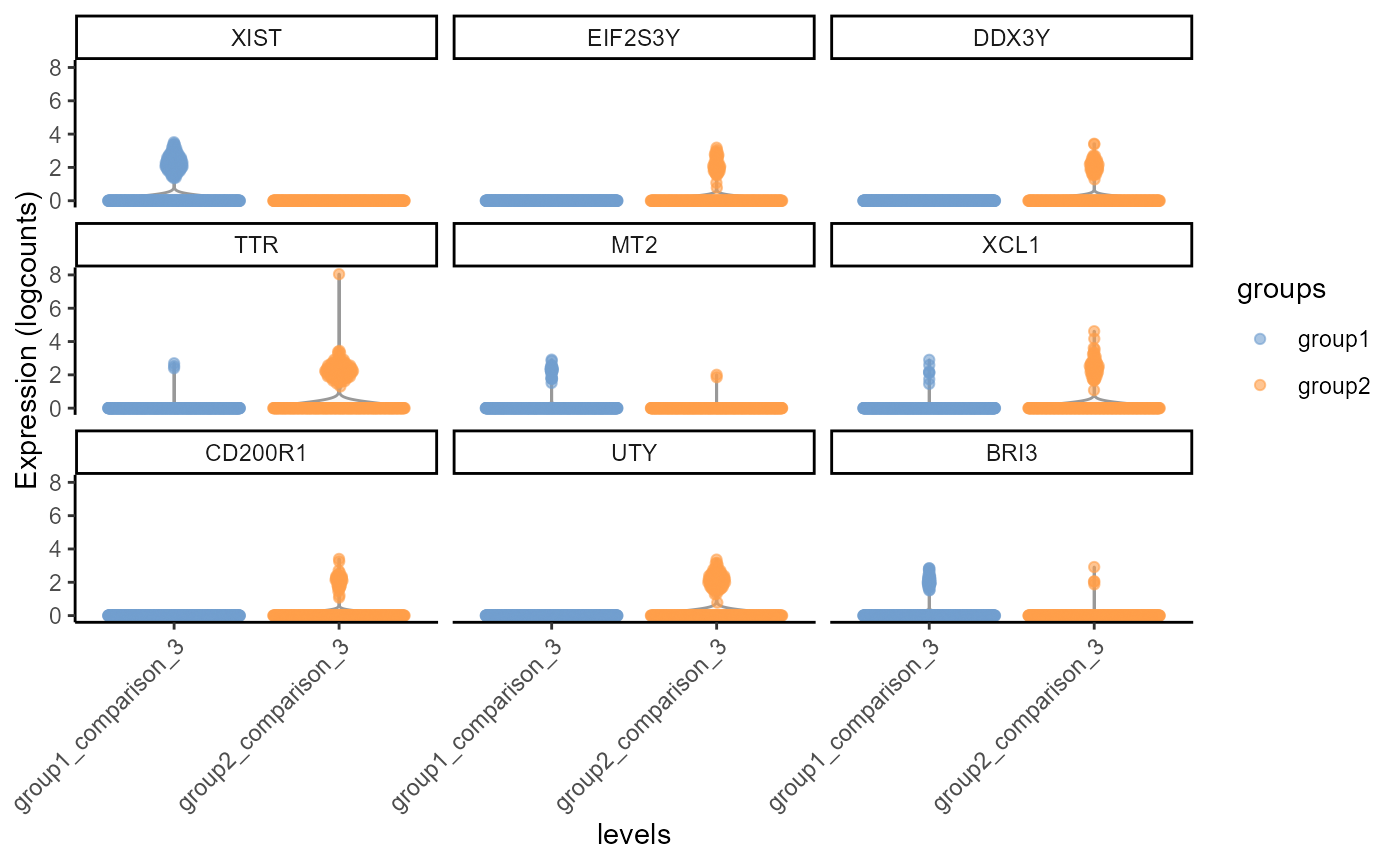
Violin Plot, including differential gene expression of of top 9 differentially expressed genes of sample 1 (group1) against sample 4 (group2), testing cells belonging to cluster 3 only.
gs <- top_gs[["comparison_5"]]  # get top gene-hits for cluster k
cs <- cs_by_k[["comparison_5"]] # subset cells assigned to cluster k
comparison_5.fig<-scater::plotExpression(input[,cs], features = gs,
        x = "levels", colour_by = "groups", ncol = 3) +
        guides(fill = guide_legend(override.aes = list(size = 5, alpha = 1))) +
        theme_classic() + theme(axis.text.x = element_text(angle = 45, hjust = 1))

plot(comparison_5.fig) 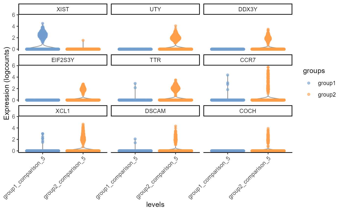
Violin Plot, including differential gene expression of of top 9 differentially expressed genes of sample 1 (group1) against sample 4 (group2), testing cells belonging to cluster 5 only.
##3.2 Heatmap
#to match ms matrix with the summary file of pseudo_DE, a new column needs to be created
pseudo_DE[["summary"]]$grouping<-rep(0,length(pseudo_DE[["summary"]][,1]))
for(k in 1:length(pseudo_DE[["summary"]][,1])){
    pseudo_DE[["summary"]]$grouping[k]<-paste(c( pseudo_DE[["summary"]]$sample_id[k], as.character(pseudo_DE[["summary"]]$comparison[k])), collapse = "_")
 }

g <- input@colData[, c( "sample_id","comparison")]
ms <- aggregate.Matrix(t(input@assays@data@listData$logcounts),
    groupings = g, fun = "mean")
ms<- SingleCellExperiment(assays = t(ms))

#To better highlight relative differences across conditions, construct the helper-function z_norm that applies a z-normalization to normalize expression values to mean 0 and standard deviation 1:

z_norm <- function(x, th = 2.5) {
    x <- as.matrix(x)
    sds <- rowSds(x, na.rm = TRUE)
    sds[sds == 0] <- 1
    x <- t(t(x - rowMeans(x, na.rm = TRUE)) / sds)
    #x <- (x - rowMeans(x, na.rm = TRUE)) / sds
    x[x >  th] <-  th
    x[x < -th] <- -th
    return(x)
}

#plotting function
plot_diff_hm <- function(ms, gs, ei) {
    mat <- ms@assays@data@listData[[1]][gs, ]
    m <- match(colnames(mat), pseudo_DE[["summary"]]$grouping)
    cols <- scales::hue_pal()(nlevels(ei$groups))
    names(cols) <- levels(ei$groups)
    col_anno <- ComplexHeatmap::columnAnnotation(
        df = data.frame(group_id = ei$groups[m]),
        col = list(groups = cols),
        gp = grid::gpar(col = "white"),
        show_annotation_name = FALSE)
    ComplexHeatmap::Heatmap(z_norm(mat),
        #column_title = k,
        name = "z-normalized\nexpression",
        col = c("royalblue", "cornflowerblue", "white", "gold", "orange"),
        cluster_rows = FALSE,
        cluster_columns = FALSE,
        row_names_side = "left",
        rect_gp = gpar(col = "white"),
        top_annotation = col_anno)
}

# plot
heatmap_pb<-plot_diff_hm(ms, top_gs$common, pseudo_DE[["summary"]])  # render differential heatmap
plot(heatmap_pb)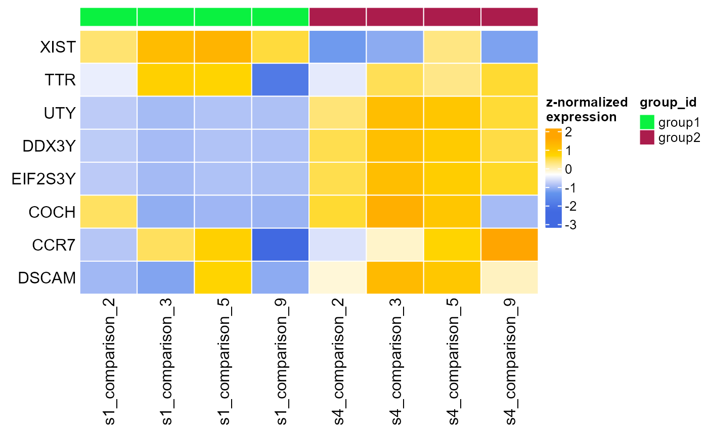
Heatmap, displaying normalised gene expression of of top 10 differentially expressed genes for each combination of samples (group) and clusters (comparison) analysed